Editing a Worksheet

The dialogs for editing a worksheet offer the same selections and features that you use to create a worksheet or workbook.

Click to learn how
To edit a worksheet:
To add an item to the current worksheet:
To delete an item from the current worksheet:

See also
Changing a Worksheet's Layout
Creating a New Workbook
Saving a Workbook
Refreshing Data in a Workbook
Deleting a Workbook


To edit a worksheet:

1. Open the worksheet that you want to edit.

2. Click the Edit Sheet icon on the toolbar, or choose Sheet | Edit Sheet.

   The Edit Sheet dialog appears.

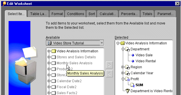
The tabs across the top of the dialog are for editing the various features of the worksheet. Clicking on a tab displays the options for the feature. For example, when the Select Items tab is selected, the items shown in the Selected list are the items currently in use on the worksheet. Items in the Available list can be added to the worksheet unless they are grayed out.

The figure above is for editing a tabular worksheet. A similar dialog appears for crosstab worksheets, except Table Layout tab becomes Crosstab Layout and the dialog does not include the Sort tab. To sort crosstab data, choose Tools | Sort.

Adding and Deleting Items on a Worksheet

The first tab on the Edit Sheet dialog is for adding or deleting items on a worksheet. For example, if the original item on the worksheet is Region, but does not include City names, you can add an item for the cities within the regions.

Adding a new item to a worksheet adds a column to the table or a row or column to a crosstab.

See also:
Editing a Worksheet
Changing a Worksheet's Layout
Saving a Workbook
Refreshing Data in a Workbook
Deleting a Workbook


To add an item to the current worksheet:

1. Click the plus (+) sign next to folders and items to see their contents.

2. Select the item in the Available list.

3. Click the Right Arrow button or drag the item to the Selected list.

   
   To delete an item from the current worksheet:

1. Select the item in the Selected list.

2. Click the Left Arrow button.

You can also delete items from a worksheet using the Table Layout tab or the Crosstab Layout tab. Click on the item then press the Delete key.

Changing a Worksheet's Layout

You can rearrange and pivot the page items, axis items, and columns on a worksheet by editing the layout.

1. Open the worksheet that you want to edit.

2. Click the Edit Sheet icon on the toolbar, or choose Sheet | Edit Sheet.

3. Click the Table Layout tab or Crosstab Layout tab. The layout shows the current arrangement of the items on the worksheet.

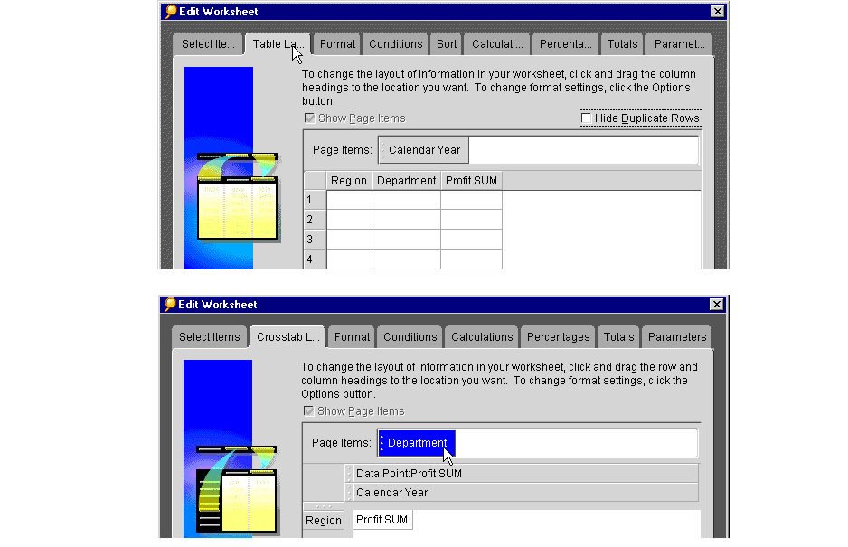
   The following examples show the Table Layout and the Crosstab Layout.

4. Select one of the items on the layout.

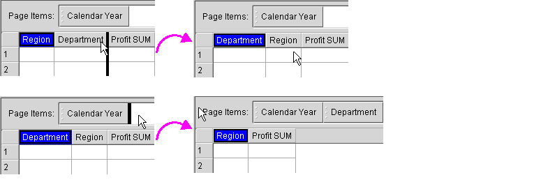
5. Drag the item to its new position on the layout. A black line on the top/bottom/side of an adjacent item shows where the items will be located when you release the mouse button.

6. Release the mouse button when the item is in its new position.

7. To delete an item from the layout, select it and click the Delete key on the keyboard.

The following examples on the Table layout show:

• moving the Region column to the right to become the second column on the worksheet

• pivoting the Department item from a column to become a Page Item.

  
  

If the worksheet contains rows with duplicate data you can hide those rows by clicking the option, Hide Duplicate Rows.

To remove the Page Items box from the top of the worksheet, drag all items from that box to the report body, then uncheck Show Page Items.

Formatting Text, Numbers, and Dates

The Workbook Wizard provides the Format Panel to help you customize the way text, numbers, and dates appear in your worksheets. You can change font size, color, and alignment one column at a time or one row at a time. You can even select multiple items to format simultaneously.

You can format the data in your worksheets, format row and column headings, and change the way an item's name displays in a worksheet. For example, you can increase the font size for a grand total row to make it more prominent. You can change the alignment of row and column headings so that they are centered or right-justified. And you can change an item's heading to something more meaningful to you; for example, you can change the heading "Profit SUM" to "Total Annual Profit".

The formats you create using the Format Panel apply to one worksheet at a time. To set default formats for all worksheets, see "Setting Sheet Format Options" and "Setting Default Format Options".

Click to learn how

To change the format of worksheet data:

To change the format of row and column headings:

To change a heading's heading:

See also:

Changing a Worksheet's Layout

To change the format of worksheet data:

1. With a workbook open, click on the tab for the worksheet that you want to format.

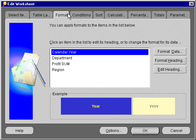
2. From the Sheet menu, choose Format... The Format Panel of the Workbook Wizard appears.

3. In the list box on the left, click the items that you want to format. You can format one item at a time or format multiple items. The Example box shows you the item's current heading format.

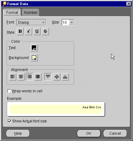
4. Click the Format Data button to change the way worksheet data appears in cells, for example, to change the font size, color, and alignment of numbers. The Format Data dialog appears.

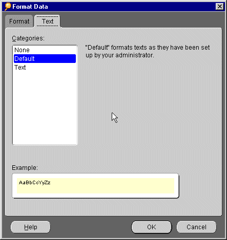
5. In the Format Data dialog, do any of the following:
   • Click the Size drop-down menu to increase or decrease the font size for data.

   • Click one or more of the Style buttons to make your data bold, italic, underlined, or strike-through.

   • Click the icons next to Text and Background to choose their colors from a color palette.

   • Click one horizontal alignment button and one vertical alignment button to change the way data is aligned within worksheet cells.

   • Click the Wrap words in cell checkbox if you want long words to be visible inside a single cell.

   • Click the Show Actual font size checkbox if you want to preview your changes in the Example box using the font size as well as the other changes that you chose above.

6. Do one of the following:
   • If the item you are formatting contains numbers (for example, currency or percentages), you will also see a tab labelled Number on the Format Data dialog. Click the Number tab to add or remove decimal places, to show or hide a currency symbol for your country, or to create a custom number format.

     NOTE: The currency symbol displayed is determined by the Country setting. To change the currency symbol, close Discoverer, then click the Choose a Language option at the Discoverer Start Page. Then follow the screen instructions for starting Discoverer, and choose a different Country setting.

   • If the item you are formatting contains dates (for example, Year or Quarter), you will also see a tab labelled Date on the Format Data dialog. Click the Date tab to change how dates appear in your worksheet.

   • If the item you are formatting contains text (for example, Region), you will also see a tab labelled Text on the Format Data dialog. Click the Text tab to change the text's capitalization to UPPERCASE, lowercase, or Capitalized.

   

   7. Preview your changes in the Example box, and then click OK. You return to the Format Panel, where you can also format row and column headings or change the way an item's name is displayed in a worksheet.

   
   To change the format of row and column headings:
   1. With a workbook open, click on the tab for the worksheet that you want to format.

   2. From the Sheet menu, choose Format... The Format Panel of the Workbook Wizard appears.

   

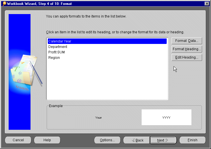
   3. In the list box on the left, click the item that you want to format. You can format the heading for one item at a time or format multiple headings. The text inside the Example box shows you the item's current heading formatting.

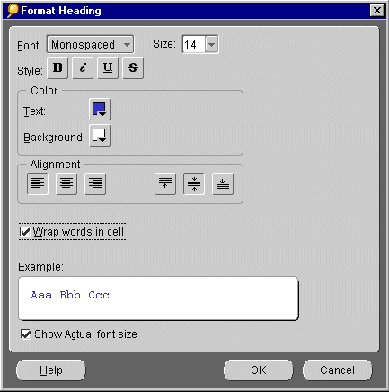
   4. Click the Format Heading button to change the way row and column headings appear on the worksheet. For example, the change the font size, color, and alignment of headings. The Format Heading dialog appears.

   

   5. In the Format Heading dialog, do any of the following:
      • Click the Size drop-down menu to increase or decrease the font size for headings.

      • Click one or more of the Style buttons to make your headings bold, italic, underline, or strike-through.

      • Click the icons next to Text and Background to choose their colors from a color palette.

      • Click one horizontal alignment button and one vertical alignment button to change the way headings are aligned within columns or rows.

      • Click the Wrap words in cell checkbox if you want long headings to be visible inside a single cell.

      • Click the Show Actual font size checkbox if you want to preview your changes in the Example box.

   6. On the Format Heading dialog, you will also see a tab labelled Text. Click the Text tab to change the heading's capitalization to UPPERCASE, lowercase, or Capitalized.

   

   7. Preview your changes in the Example box, and then click OK. You return to the Format Panel, where you can also format worksheet data or change a item's heading.

   
   To change a heading's heading:
   1. With a workbook open, click on the tab for the worksheet that you want to format.

   2. From the Sheet menu, choose Format... The Format Panel of the Workbook Wizard appears.

   

   3. In the list box on the left, click the item that you want to edit.

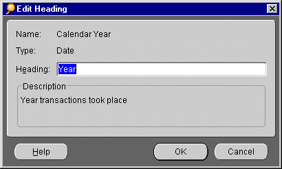
   4. Click the Edit Heading button to change the way an item's name appears on the worksheet; for example, to change the heading Calendar Year to Year. The Edit Heading dialog appears.

   

   5. In the Heading text box, type a new name for this item.

   6. Click OK. You return to the Format Panel, where you can also format worksheet data and format row and column headings.